For my final project in my Data Science class, I decided to investigate something I always wondered about - music and its relation to popular taste! Here’s my attempt to answer the billion dollar question: what makes a popular song?

Introduction

But to be more specific, here I am aiming to predict the popularity of a song based on its audio features. Specifically, I used extract data from 19000 songs on Spotify using Spotify’s in-built API¹, and analyzed each track’s structure and musical content, including tempo, acousticness, duration etc. Specifically, we define our variables:

• Popularity: Calculated by algorithm (total number of plays/how recent plays are) – between 0 and 100, with 100 being the most popular.
• Tempo: The overall estimated tempo of the section in beats per minute (BPM).
• Key: The estimated overall key` of the section.
• Mode: Indicates the modality (major or minor) of a track, the type of scale from which its melodic content is derived.
• Acousticness: A confidence measure from 0.0 to 1.0 of whether the track is acoustic. 1.0 represents high confidence the track is acoustic.
• Danceability: Danceability describes how suitable a track is for dancing based on a combination of musical elements including tempo, rhythm stability, beat strength, and overall regularity. A value of 0.0 is least danceable and 1.0 is most danceable.
• Energy: Energy is a measure from 0.0 to 1.0 and represents a perceptual measure of intensity and activity. Perceptual features contributing to this attribute include dynamic range, perceived loudness, timbre, onset rate, and general entropy.
• Instrumentalness: Predicts whether a track contains no vocals. “Ooh” and “aah” sounds are treated as instrumental in this context. Rap or spoken word tracks are clearly “vocal”.
• Liveliness: Detects the presence of an audience in the recording. Higher liveness values represent an increased probability that the track was performed live.
• Speechiness: Detects the presence of spoken words in a track. The more exclusively speech-like the recording (e.g. talk show, audio book, poetry), the closer to 1.0 the attribute value.

Model

Data

Data was extracted from Spotify and loaded into pandas using a dataframe, categorized by genre. Songs were grouped by their popularity and the mean for each (numerical) feature was calculated. Preliminary analysis revealed that Classical music held the strongest single-variable linear correlations with popularity, and thus further analysis was performed using the Classical music dataset of 7929 songs.

The original dataset used can be found here. In this small project, we only used classical songs and didn’t analyze songs belonging to other genres - however, the same analysis process still holds!

# import libraries
import numpy as np
from scipy import stats as st
import pandas as pd
import seaborn as sns
import matplotlib.pyplot as plt
import statsmodels.formula.api as smf
import statsmodels as sm
import sklearn as skl
import sklearn.metrics as skm

# reading in data
projectData = pd.read_csv("SpotifyFeatures.csv").drop(['track_id', 'valence'],\
             axis = 1)
classicalData = projectData[projectData['genre']=='Classical']
classicalData = classicalData[classicalData.popularity >= 10]

# preliminary data analysis, pairplot to find variables with correlation
classicalMean = classicalData.groupby(['popularity']).mean()
classicalMean['popularity']=classicalMean.index

CDM1 = sns.pairplot(classicalMean,y_vars=["popularity"],x_vars=["acousticness","danceability","duration_ms","energy","instrumentalness"],kind="reg")
CDM1.set(ylim=(-10, 100))
CDM2 = sns.pairplot(classicalMean,y_vars=["popularity"],x_vars=["liveness","loudness","speechiness","tempo"],kind="reg")
CDM2.set(ylim=(-10, 100))
plt.show()

Fitting

Looks promising! Let’s try fitting a multivariate linear regression model to our data. To avoid overfitting, the data was split into training and test sets. The statsmodels.formula.api’s Ordinary Least Squares Regression model was fitted using training data, with popularity as the predictor and variables with the strongest linear correlations from before.

# splitting up data into training and testing set
trainFraction = .30
sample = np.random.uniform(size = classicalData.shape[0]) < trainFraction

classicalTrain = classicalData[sample]
classicalTest = classicalData[~sample]

# modeling popularity with OLS model
classicalTrainMean = classicalTrain.groupby(['popularity']).mean()
classicalTrainMean['popularity']=classicalTrainMean.index

results = smf.ols('popularity ~ acousticness + speechiness + instrumentalness + liveness', data = classicalTrainMean).fit()
print(results.summary2())

Some quick analysis

For our OLS mode, the coefficients for each variable were obtained from minimizing \[\sum ({Popularity}-\beta_0-\beta_1 x_{acoustic}-\beta_2 x_{speech}-\beta_3 x_{instru}-\beta_4 x_{live})^2 \]

The interpretation of the regression coefficient is the estimated expected change in the outcome for a single unit change in the regressor with all other regressors held constant i.e. for \(\beta_1\), it is the estimated change in popularity for a single unit change in acousticness. From our model’s fit, we have:

\[\beta_0=104.0,\beta_1=59.02,\beta_2=-143.6,\beta_3=33.39,\beta_4=-185.6\]

                   Results: Ordinary least squares
=====================================================================
Model:                OLS               Adj. R-squared:      0.568   
Dependent Variable:   popularity        AIC:                 448.9744
Date:                 2019-10-06 21:40  BIC:                 459.2766
No. Observations:     58                Log-Likelihood:      -219.49 
Df Model:             4                 F-statistic:         19.74   
Df Residuals:         53                Prob (F-statistic):  5.34e-10
R-squared:            0.598             Scale:               124.06  
---------------------------------------------------------------------
                   Coef.   Std.Err.    t    P>|t|    [0.025   0.975] 
---------------------------------------------------------------------
Intercept         104.0369  18.9055  5.5030 0.0000   66.1174 141.9565
acousticness      -59.0218  18.1056 -3.2599 0.0020  -95.3370 -22.7066
speechiness      -143.6381 131.5060 -1.0923 0.2797 -407.4058 120.1296
instrumentalness   33.3890  12.5054  2.6700 0.0100    8.3064  58.4716
liveness         -185.6042  47.3051 -3.9236 0.0003 -280.4861 -90.7222
---------------------------------------------------------------------
Omnibus:               0.959          Durbin-Watson:            0.494
Prob(Omnibus):         0.619          Jarque-Bera (JB):         1.001
Skew:                  -0.196         Prob(JB):                 0.606
Kurtosis:              2.489          Condition No.:            134  
=====================================================================

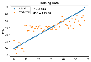
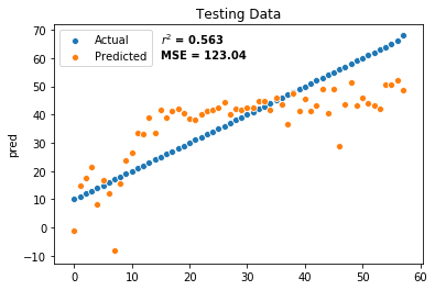
Predicted popularities were evaluated using the model on both the training and test set, and the mean squared error was evaluated. Results predicted from the training set and the testing set achieved \(r^2\) coefficients of 0.598 and 0.563, and MSE of 113.36 and 123.04 respectively.

Key and Mode

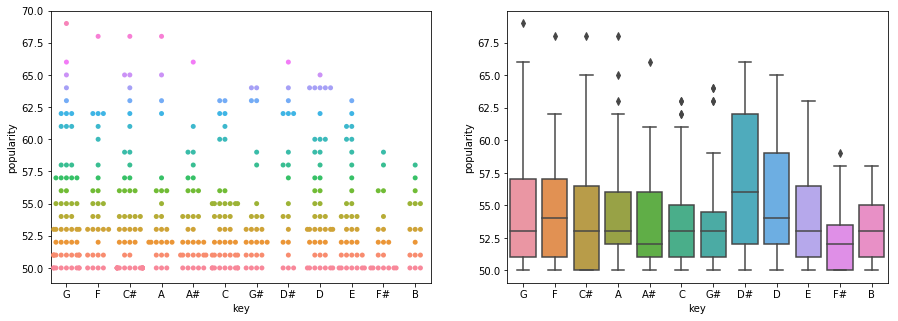
# looking at most popular keys and modes
classicalPopData = classicalData[classicalData.popularity >= 50]

fig, ax = plt.subplots(1,2,figsize=(15,5))
d=sns.swarmplot(x="key", y="popularity", hue="popularity", data=classicalPopData, ax=ax[0])
d.legend_.remove()
sns.boxplot(x="key", y="popularity", data=classicalPopData, ax=ax[1])
fig.show()

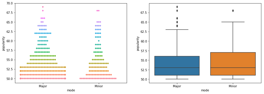
fig, ax = plt.subplots(1,2,figsize=(15,5))
d=sns.swarmplot(x="mode", y="popularity", hue="popularity", data=classicalPopData, ax=ax[0])
d.legend_.remove()
sns.boxplot(x="mode", y="popularity", data=classicalPopData, ax=ax[1])
fig.show()

# no clear trend here! ):

Interpretation

Thus, we have obtained a model that predicts a Classical song’s popularity relatively accurately based on song metrics such as acousticness, speechiness, instrumentalness and liveness. It may thus be possible to predict the popularity of a new (Classical) song on spotify by analyzing the metrics and using the model. From the model, it appears that less speech and liveness (i.e. a better recording) and greater instrumentation tends to correlate with a higher popularity. However, we do note that the model only applies to a subset of songs – specifically, I removed songs with less than 20 popularity from analysis, in other to obtain a less skewed distribution of song popularity. In addition, an OLS model is one of the simplest models that may not be able to accurately model a complicated function such as song popularity right. We can consider using other models, such as a Logistic Regression, PCA or even some unsupervised learning models! Lastly, this form of analysis can also be applied to the other 26 song genres in the data set, to identify any interesting trends.